Fokus | How we model football team strength

On 4 November, Viking host Sabah FK in the Champions League. Sabah arrive as champions of Azerbaijan. That title shows how they performed in their domestic competition. It does not tell Viking how that level compares with Eliteserien, or whether Sabah's strength lies in their attack or defence. This is the problem we are solving through the team strength model.

These problem statements are practical questions when preparing for an unfamiliar opponent. Yet, identifying the clubs' relative strengths is easier said than done. The final table position reflects points earned against different clubs, in competitions with varying strengths, scoring patterns and style. European matches across leagues help connect the relative level of the league, but they provide only a small sample of the total games played.

Recruitment has the same need for context. A player's numbers are shaped by the strength of the club, the opponents, and the league around them. Before comparing players from different competitions, recruitment teams need to understand the level at which those performances were produced.

We built this model to provide that reference. It estimates the level underneath the results, separates attack from defence, and puts clubs from different leagues on the same scale. This gives more context and a stronger starting point for match analysis and player evaluation across clubs and leagues.

What the league tables fail to tell you

Take Eliteserien after 25 matches. Viking and Bodø/Glimt are level on points and goal difference. The league table is a good overview of the season, and an expected points table is a good overview of the performances behind it. Points record the results. Expected points record what the sum of the chances in each match is usually worth in terms of points achieved.

Team strength is our estimate of a club's ability to score and prevent goals, after accounting for the opponents in the league, home advantage and recency of evidence.

Eliteserien table after 25 matches — Eliteserien after 25 matches.

We use our model to compare each club with an average club from its own league on neutral ground. How many goals would we expect it to score, and how many to concede? The opponent is hence assumed to be the same for every club, so the specific fixture list is not a part of the comparison. Higher on the chart means a better attack. Further right means fewer goals conceded and a better defence. The two lines mark the league average. Clubs in the top-right area rate above average at both ends of the pitch.

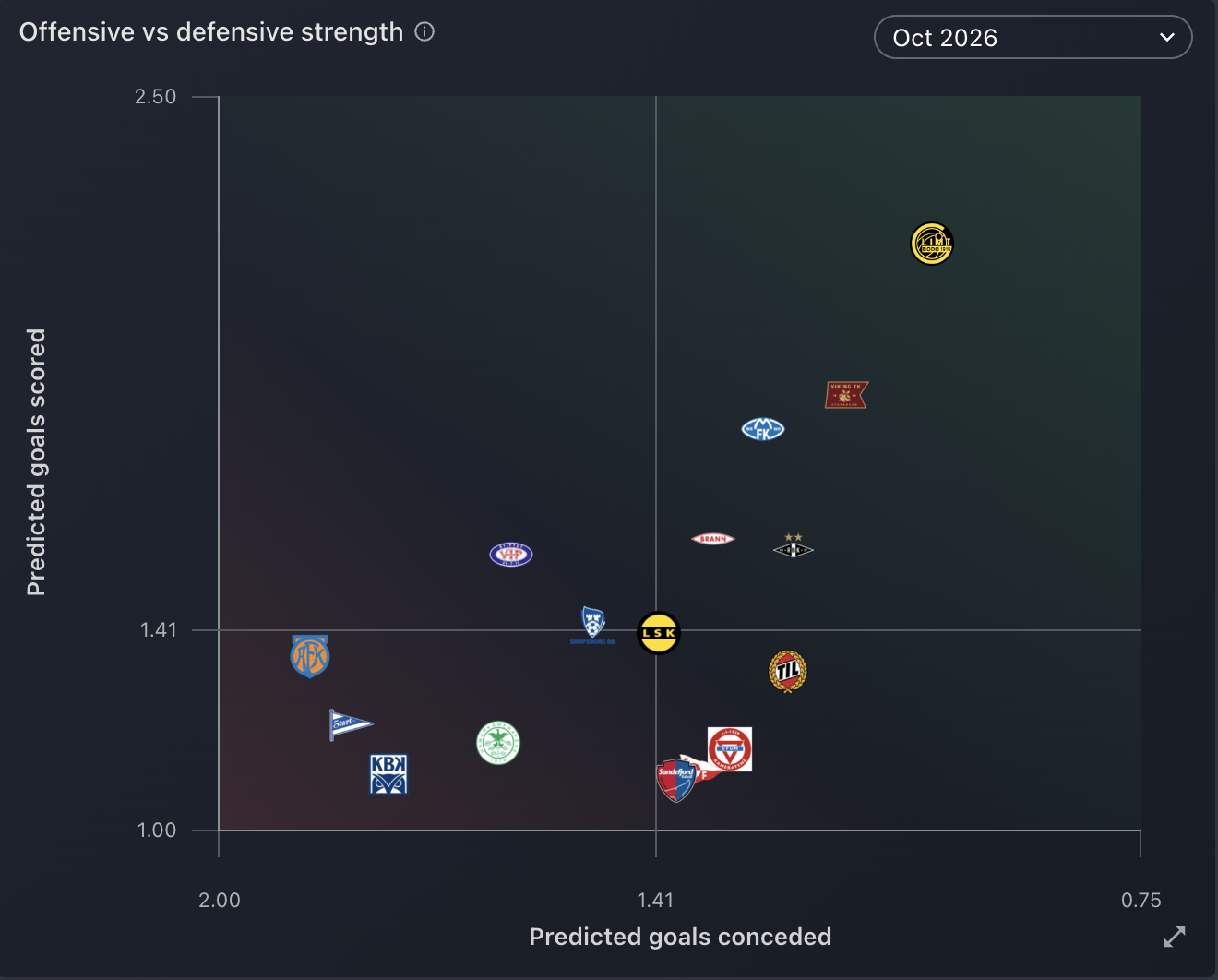
Eliteserien clubs by expected goals scored and conceded, November 2026 — Attack-defence plot for clubs in Eliteserien, 1 November 2026. Each logo shows expected goals scored and conceded against an average Eliteserien opponent on neutral ground.

Bodø/Glimt and Viking are level on points. The plot puts Bodø/Glimt ahead at both ends. Against an average Eliteserien side on neutral ground on 1 November 2026, Bodø/Glimt are expected to score 2.20 goals and concede 1.03. Viking are expected to score 1.89 and concede 1.15.

Inside Eliteserien the positions can be compared directly. Every club is measured against the same league average. Two clubs can also sit close overall and still be different sides. One may overwhelm others in attack. The other may concede almost nothing.

The rest of the post builds these numbers from the inside out. We start by estimating how often each side should score. Then we separate what belongs to the club from what belongs to the league, and decide how far the available evidence should move the estimate.

Starting with goals

To understand a club's strengths, we start with its match history: the goals it scored, the goals it conceded, and the opponents it faced. From that history, the model estimates how often each side is likely to score in a given match.

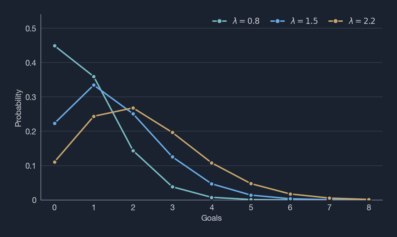
A club can score zero goals, one goal, two goals, three goals, and so on. The Poisson distribution turns one number, the expected scoring rate, into a probability for each of those counts.

A rate of 1.5 can describe how likely zero, one, two, and three goals are. Zero, one, two or three goals all have a real chance of occurring, but their probability varies. A higher rate shifts the distribution toward bigger scorelines.

One rate describes only one club. A match needs two: one for the home team and one for the away team. Given those rates, the Poisson distribution gives a probability for every scoreline. The hard part is estimating the rates.

Poisson probabilities for scoring rates 0.8, 1.5 and 2.2 — Poisson probabilities for three scoring rates, $\lambda = 0.8$ , 1.5 and 2.2. The horizontal axis is goals scored, from 0 to 8, and the vertical axis is probability. At $\lambda = 0.8$ the most likely outcome is 0 goals, at 1.5 it is 1 goal, and at 2.2 it is 2 goals.

Formula: Poisson

The Poisson distribution has one parameter, $\lambda$ , the expected scoring rate.

P(X = k) = e^{-\lambda} \frac{\lambda^{k}}{k!}

For $\lambda = 1.5$ , zero, one, and two goals all carry meaningful probability. As $\lambda$ increases, the mass of the distribution moves toward higher scorelines.

Independence, conditional on the two rates, means the scoreline probability is the product of the two Poisson probabilities.

P(H = h,\ A = a) = P(H = h)\, P(A = a)

A home win is the sum of those probabilities over scorelines with more home goals. A draw sums the equal scorelines. An away win sums the rest.

Goals tell us the score. Expected goals give another view of the chances that produced it. One deflection or one exceptional finish can separate the two.

Two clubs can both win 1-0 and have produced very different matches. One creates six good chances and controls the game. The other scores with its only real attempt and spends the rest of it defending. Treating those as the same performance overlooks important information from the game.

Hence, where we have the information of xG, we blend the xG with the actual goals scored by a club, to give more context to the underlying performance in the game. Where xG is missing, the model uses the scoreline alone. That matters in a global model because data coverage varies widely between competitions and seasons.

Formula: xG blend

When xG is present, the match target is a weighted blend. Otherwise the target is the goal count.

y = w\,\mathrm{xG} + (1 - w)\,\mathrm{goals}

That target can sit between two integers. The Poisson fit uses it directly, through the gamma function in place of the factorial.

\ell = y\log\lambda - \lambda - \log\Gamma(y + 1)

The aim is to reduce how much our estimate of a club's strength depends on whether its chances happened to be converted in a particular match.

Attack against defence

One overall rating for each club would hide too much. We therefore estimate attack and defence separately. Every match gives us two contests: the home attack against the away defence, and the away attack against the home defence. A higher defensive rating means a stronger defence, so it reduces the opponent's expected scoring rate.

We also separate the effect of playing at home from the strength of the club. Otherwise some of the venue's advantage could be mistaken for a stronger attack or a weaker opponent. When we compare clubs on neutral ground, we can switch that home effect off.

A club's results only make sense in context. The same record can mean something different in a stronger league, while some leagues simply produce more goals than others. We call those two parts league strength and league pace. Pace here means the league's scoring environment.

With that context in place, we can compare a club's attack and defence with a typical club from its own league. But being strong relative to your own league is not enough: the level of the league itself also matters.

Formula: scoring rates

For a match between home team h and away team a, the expected scoring rates are

\begin{aligned} \lambda_{h} &= \exp(\mu + \eta_m + \mathrm{attack}_{h} - \mathrm{defence}_{a}) \\ \lambda_{a} &= \exp(\mu + \mathrm{attack}_{a} - \mathrm{defence}_{h}) \end{aligned}

Attack and defence are built from a league part and a club part.

\begin{aligned} \mathrm{attack}_{i} &= S_{L} + P_{L} + u_{\mathrm{atk}, i} \\ \mathrm{defence}_{i} &= S_{L} - P_{L} + u_{\mathrm{def}, i} \end{aligned}

$\mu$ is the baseline scoring level. The model works on a log scale, so $\exp(\mu)$ is the baseline expected scoring rate before club, league, or match effects.

$\eta_m$ is home advantage. League matches, domestic cups, and continental matches use different values. On neutral ground the term is left out.

$u_{\mathrm{atk}}$ and $u_{\mathrm{def}}$ are how the club differs from its league reference. $S_{L}$ is league strength. $P_{L}$ is league pace. The exponential turns the combined effects into a positive expected scoring rate.

League strength and league pace are different things

This distinction matters. A league can be strong and low-scoring, or open and ordinary. Strength is the quality. Pace is the scoring environment.

Consider two pairs of leagues that our model rates at a similar level: Serie A and the Bundesliga, and the Greek Super League and the Swiss Super League. Within each pair, one league produces more goals. The model records that as pace. Clubs can then be compared across leagues on strength, while the more open competition shows up in its scoring environment.

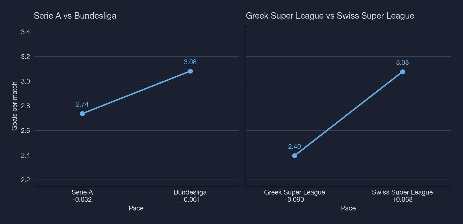
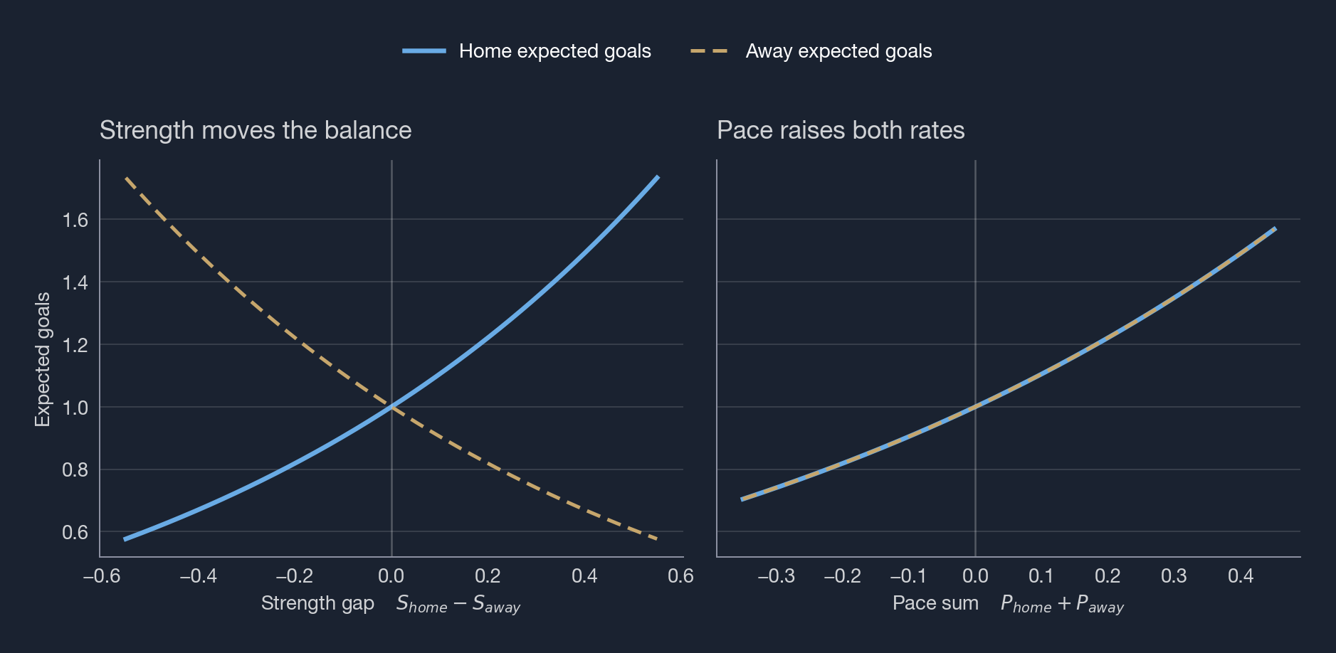
Observed total goals per match in Serie A, the Bundesliga, the Greek Super League, and the Swiss Super League — Observed goals per match, home plus away, averaged over every played match in that league. The leagues in each pair have similar estimated strength and different pace, so their matches finish with different totals.

Strength changes the balance between two opponents. When a club from a stronger league meets one from a weaker league, all else equal, we expect the stronger-league club to score more and concede less. Each club's own attack and defence are what leave room for exceptions. Pace moves both clubs' scoring rates together. A meeting between two high-scoring leagues can produce a more open game without either side receiving a strength bonus.

Home and away expected goals as league strength and league pace change — Expected goals for the home side (solid) and the away side (dashed) as league strength and league pace change, with all other effects set to zero and home advantage excluded. Left: as the strength gap between the home and away leagues grows, the home rate rises and the away rate falls, and they cross at equal strength. Right: as the combined pace of the two leagues rises, both rates increase together, and the two lines lie on top of each other. Strength moves the balance between the clubs. Pace moves the scoring level for both.

Formula: strength and pace

In the home scoring rate, league strength enters as a difference.

S_{h} - S_{a}

A stronger home league makes the term positive. A weaker home league makes it negative. For the away team the sign flips.

S_{a} - S_{h}

Pace enters as a sum, and the same sum appears in both scoring rates.

P_{h} + P_{a}

When two clubs from the same league meet, the strength terms cancel.

S_{L} - S_{L} = 0

A domestic league match tells us about the clubs and about the scoring environment. Relative league strength comes from matches that connect competitions, such as cross-tier domestic cups and continental matches.

Pace stays in the rate. For two clubs from the same league

P_{L} + P_{L} = 2P_{L}

Domestic league matches carry most of the information about a league's scoring pace. If matches in a competition keep producing more or fewer goals than the rest of the model expects, that shows up in the league's pace.

Matches between leagues establish how strong the leagues are relative to each other. Matches inside a league establish much of the scoring environment.

A club's strength is relative to its league

League strength, league pace, and each club's attack and defence are estimated together. The league terms give every club a reference. The club terms measure how far its attack and defence sit from a typical side in that league.

League matches separate clubs inside the same competition, but cannot by themselves establish the level of the competition. When two clubs from the same league meet, the league-strength term is the same on both sides and cancels out. Cross-league matches provide the missing link. The Norwegian Cup connects Eliteserien with OBOS-ligaen and PostNord-ligaen, while UEFA competitions connect domestic leagues across Europe. The model estimates league levels from that network of results over time, not from a single match.

That shared reference is especially useful for promoted clubs, newly covered competitions, and clubs with only a small number of matches in the data. When the evidence is thin, the model starts conservatively. A handful of matches leaves the first estimate near the level of its league.

As matches accumulate, the results can pull the club further above or below that reference. Leagues with few matches connecting them to other competitions are treated in the same cautious way. In practice, the rating moves less where football has given the model less to work with.

The same goal raises the scorer's attack and lowers the opponent's defence. The rest of the schedule decides how the two share that goal. A club that keeps scoring against strong defences takes the attack. A club that keeps conceding to ordinary attacks takes the defence.

Match weights and the priors are in that same fit. Recent matches count more toward the underlying rating. Where the evidence is thin, the prior keeps the club near its league.

Formula: priors

With little evidence, we assume the club sits near its league. That assumption is a Gaussian prior on the club terms. For a club's first spell

\begin{aligned} u_{\mathrm{atk}} &\sim N(0,\, \sigma^{2}_{\mathrm{club}}) \\ u_{\mathrm{def}} &\sim N(0,\, \sigma^{2}_{\mathrm{club}}) \end{aligned}

The priors are centered at zero. Zero places the club at its league. League strength and pace use similar Gaussian priors, which matters most for leagues with few matches connecting them to the rest of the model.

The effect is Bayesian shrinkage. With little evidence, the club stays near its league. As the likelihood grows relative to the prior, the club can move further away.

Promotion and relegation

Promotion creates a peculiar rating problem. The club has changed leagues, and it is still the same team.

Before the move, the club is measured against the average club in its old league. If its attack or defence sits above that reference, we want to keep that level. After promotion, the reference is an average club from a stronger league.

The new rating starts from the club's previous rating and the difference between the two league baselines. The club keeps the same attacking and defensive level, but is now judged relative to the new league average. Matches in the new league then move the estimate as fresh evidence arrives.

Formula: transition prior

The club's new attack and defence, relative to the new league, are normally distributed. The centre is the previous level, adjusted by the gap between the league the club has left and the league it has joined.

\begin{aligned} u_{\mathrm{atk}}^{\mathrm{new}} &\sim N\!\left( u_{\mathrm{atk}}^{\mathrm{old}} + \kappa \big(C_{\mathrm{atk}}^{\mathrm{old}} - C_{\mathrm{atk}}^{\mathrm{new}}\big),\, \sigma^{2} \right) \\ u_{\mathrm{def}}^{\mathrm{new}} &\sim N\!\left( u_{\mathrm{def}}^{\mathrm{old}} + \kappa \big(C_{\mathrm{def}}^{\mathrm{old}} - C_{\mathrm{def}}^{\mathrm{new}}\big),\, \sigma^{2} \right) \end{aligned}

The league component differs for attack and defence.

\begin{aligned} C_{\mathrm{atk}} &= S + P \\ C_{\mathrm{def}} &= S - P \end{aligned}

$\kappa$ sets how much of the gap between the two leagues enters the centre of that normal. Promotion and relegation can use different values.

Recent matches count more

Clubs change. Players leave, coaches arrive, and tactical ideas take hold or disappear. A match from last month should therefore tell us more about the club today than a match from three seasons ago.

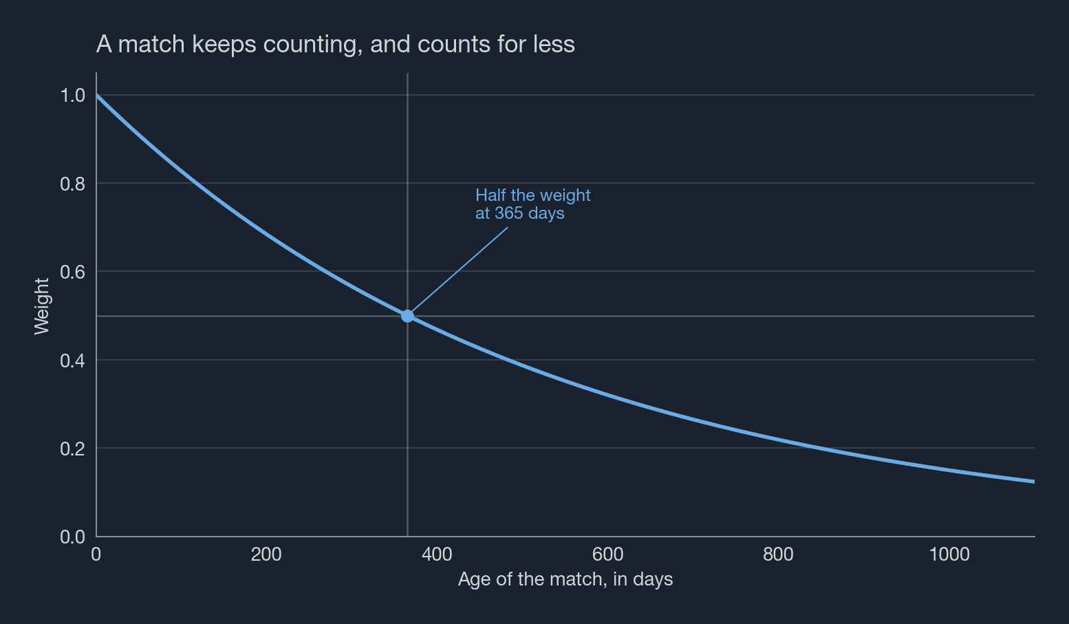
Older matches gradually lose influence. They stay in the model and matter less as time passes.

Match weight declining exponentially with age — Match weight as a function of age. A match played today has weight 1, and the weight declines exponentially over time. The implied half-life is how long it takes for a match's influence to fall by half.

Formula: time decay

The weight decays exponentially with age.

w = \exp(-\xi \cdot \text{age in days})

$\xi$ controls how quickly older matches lose influence. This weight changes how much history goes into the longer-term level. Form uses a much shorter half-life inside the same fit.

Recent matches already carry more weight, so why add form as well? Because the two mechanisms answer different questions.

Time decay decides how much each match contributes to the underlying level. A recent match matters more than an old one, but both still update the same longer-term estimate.

Form measures where the club sits relative to that underlying level right now. A strong run can lift the current rating above it, while a poor run can pull the current rating below it.

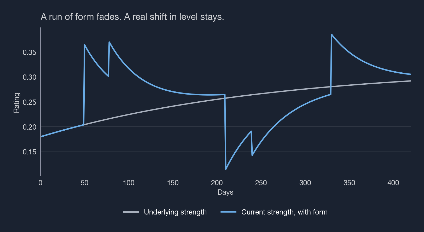
Underlying strength and current strength including form through time — Underlying strength is grey. Current strength, with form, is blue. The gap is the form adjustment.

In the figure, the grey line moves gradually as evidence accumulates. The blue line can react faster. When it rises above the grey line, recent performances have been stronger than the underlying level. Without continued evidence, the gap closes again.

This lets a recent deviation sit apart from the longer-term estimate. Sustained performances eventually move the underlying level. A brief spell mainly creates a temporary gap between the two lines.

Formula: form adjustment

Underlying strength and form are estimated together, in the same fit as the league terms. Form is a separate adjustment on attack and defence. Its prior is Gaussian and centered at zero. The underlying rating uses the slower match weights.

\begin{aligned} \mathrm{attack} &= S + P + u_{\mathrm{atk}} + f_{\mathrm{atk}} \\ \mathrm{defence} &= S - P + u_{\mathrm{def}} + f_{\mathrm{def}} \end{aligned}

$h$ is the form half-life. It discounts older matches. For a match $\textit{age}$ days old, form enters the home scoring rate through

r(\text{age}) = \exp\left(-\frac{\ln 2}{h}\,\text{age in days}\right)

\begin{aligned} \log\lambda_h = \mu + \eta_m &+ C_{\mathrm{atk}, h} + u^{\mathrm{atk}}_h - C_{\mathrm{def}, a} - u^{\mathrm{def}}_a \\ &+ r(\text{age})\left(f^{\mathrm{atk}}_h - f^{\mathrm{def}}_a\right) \end{aligned}

From continental ratings to a global scale

Club competitions create connected networks of evidence within each football confederation. Champions League matches link Norway with England, Spain, and the rest of UEFA. Similar competitions link leagues within Asia, Africa, North America, and South America. Results allow the model to compare clubs inside each network.

Once the model is fitted, every club has an attacking level and a defensive level. Their sum gives the overall rating. League pace raises the attacking level and lowers the defensive level by the same amount, so it cancels in the combined rating. League strength, the club's attack and defence, and current form remain.

Formula: overall rating

Pace is added to attack and subtracted from defence.

\begin{aligned} \mathrm{attack} &= S + P + u_{\mathrm{atk}} \\ \mathrm{defence} &= S - P + u_{\mathrm{def}} \end{aligned}

Adding the two gives

\begin{aligned} R_{\mathrm{underlying}} &= (S + P + u_{\mathrm{atk}}) + (S - P + u_{\mathrm{def}}) \\ &= 2S + u_{\mathrm{atk}} + u_{\mathrm{def}} \end{aligned}

$+P$ and $-P$ cancel. League strength and the club's attack and defence remain. Form is added to attack and defence, so it stays in the total.

R_{\mathrm{current}} = R_{\mathrm{underlying}} + f_{\mathrm{atk}} + f_{\mathrm{def}}

In a neutral match, with home advantage left out, the gap between two clubs on this rating is the gap in their log scoring rates.

\log\left(\frac{\lambda_i}{\lambda_j}\right) = R_{\mathrm{current}, i} - R_{\mathrm{current}, j}

The club with the higher rating is expected to score more and concede less against the same opponent.

These results can place clubs and leagues on a common scale within one confederation. Competitive matches between confederations are too rare to place the separate networks on a global scale from results alone.

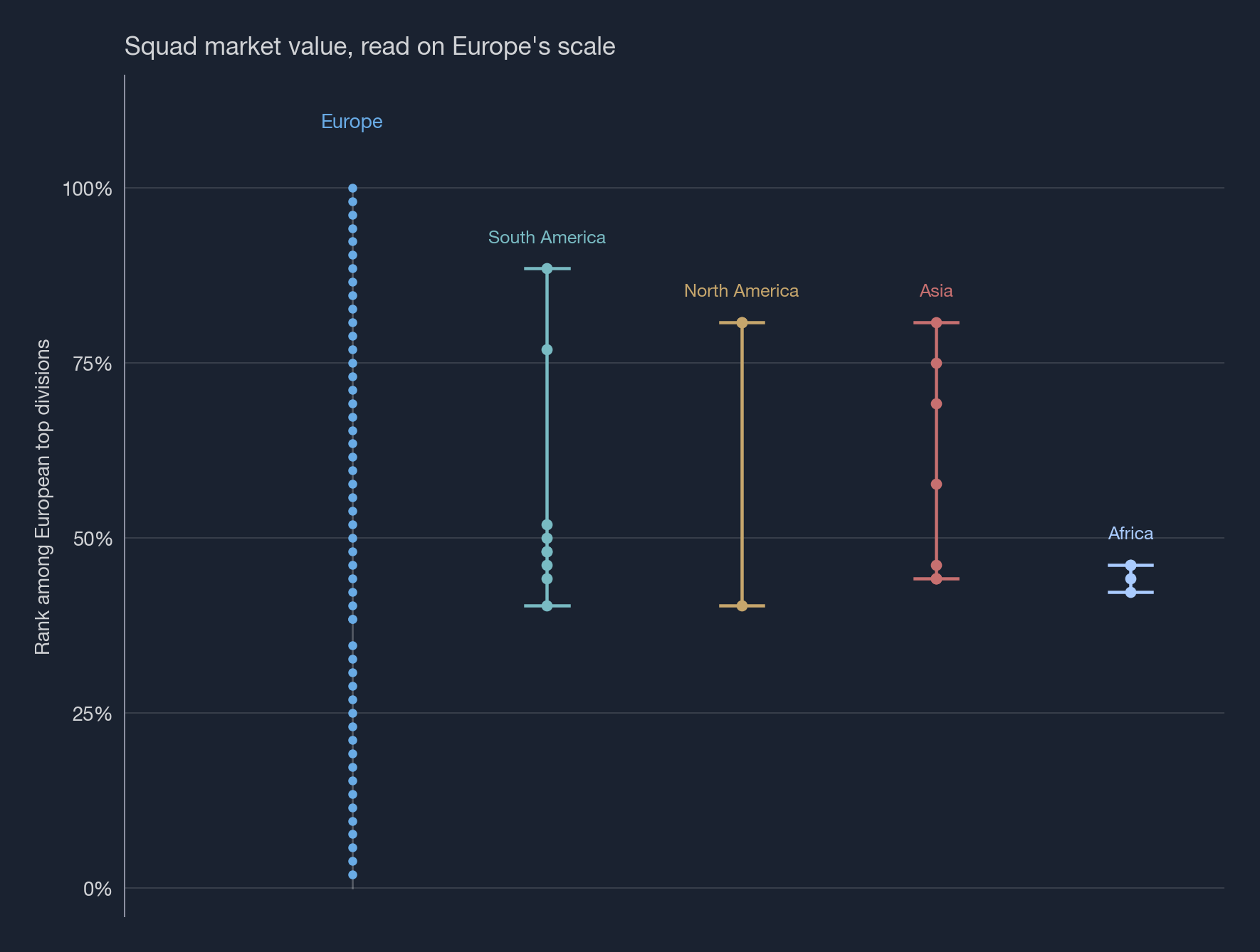
To connect those scales, we use squad market values as an external reference. For each confederation, we compare the distribution of average squad values across its top divisions with the same distribution in Europe. We then align that confederation's match-based ratings with the corresponding part of the European rating scale.

Market values do not decide which clubs are strongest within a confederation. Match results still determine the order and the differences between clubs and leagues. Market values are used only to set the cross-confederation level where direct match evidence is too sparse.

This step adds more uncertainty than a comparison within one connected competition network. Market values are an imperfect proxy and are influenced by player age, contract status, data coverage, and local transfer markets. Global ratings should therefore be read as calibrated estimates, especially when comparing clubs from different confederations.

Top divisions in Europe, South America, North America, Asia, and Africa positioned within Europe's squad market-value distribution — Each dot is a top division. Its vertical position shows where its average squad value falls within the distribution of European top divisions. Higher means closer to Europe's most valuable leagues. The vertical bars show the range covered by each confederation.

Where Eliteserien ranks in Europe

The bars are a power rating of the underlying league strength on 1 November 2026. 100, which is the strongest league, is the English Premier League. Eliteserien's strength becomes 73.2, whilst the Premyer Liqa in Azerbaijan is 59.1.

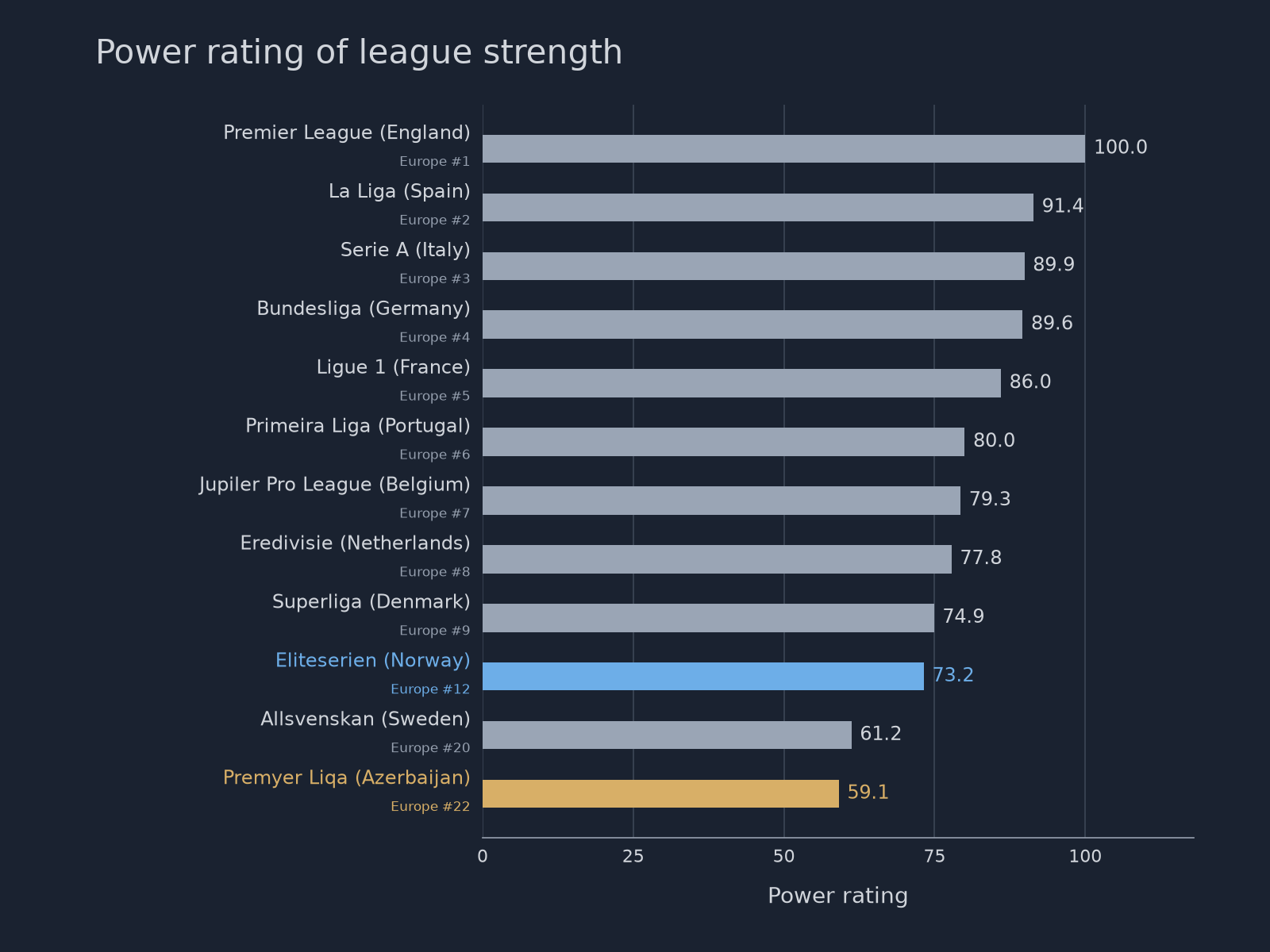
Horizontal bar chart of power ratings for 12 European top divisions. Eliteserien is Europe #12 at 73.2 and Premyer Liqa is Europe #22 at 59.1. — Fokus team strength model, 1 November 2026. Selected men's top divisions. Europe # is the rank among the 52 tier-one leagues. The power rating uses every men's domestic competition in Europe, from the weakest at 0 to the strongest at 100.

League strength is the reference for the clubs in that competition. Attack and defence then place each club above or below it. A team can rate higher than its league, or lower, depending on those two ratings.

Viking and Sabah on one scale

We can now return to the question we started with: how do Viking and Sabah compare when their domestic records come from different leagues, and where does each side's strength lie?

Eliteserien and the Premyer Liqa both sit in that European network. They do not need to meet regularly. UEFA matches connect them through other leagues and shared opponents. Across that match history, the model rates Eliteserien as the stronger competition. Sabah can therefore sit well above the average club in Azerbaijan and still start from a lower league reference than Viking.

Viking's overall rating is 1.59 and Sabah's is 1.09. Sabah's 1.09 places them 8th among the clubs in Eliteserien, just below Lillestrøm.

Sabah placed among Eliteserien clubs. Sabah has an overall rating of 1.09 and Viking 1.59. — Sabah placed among Eliteserien clubs, 1 November 2026. Sabah's overall rating is 1.09, 8th in this group, just below Lillestrøm.

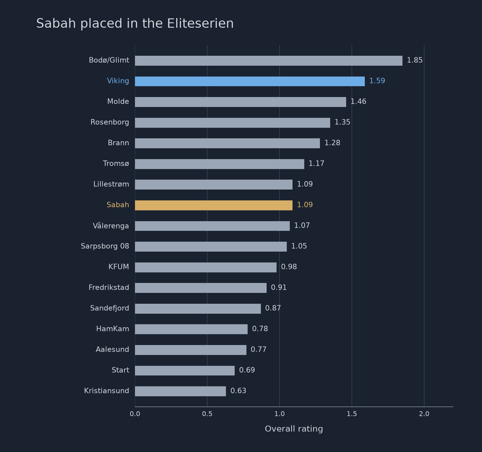
Viking's attack is rated at 0.89 and their defence at 0.70. Sabah's attack is 0.53 and their defence 0.56. Sabah's attack sits a little further above the Premyer Liqa baseline than Viking's sits above the Eliteserien baseline. The model rates Eliteserien as the stronger league, however, and the combined comparison puts Viking ahead at both ends.

The model expects Viking to score 2.24 goals and Sabah 1.07. Rounded to whole percentages, the match probabilities are 64% for a Viking win, 19% for a draw, and 17% for a Sabah win. The goal distributions peak at two goals for Viking and one for Sabah, although Sabah are almost as likely to score none as they are to score once.

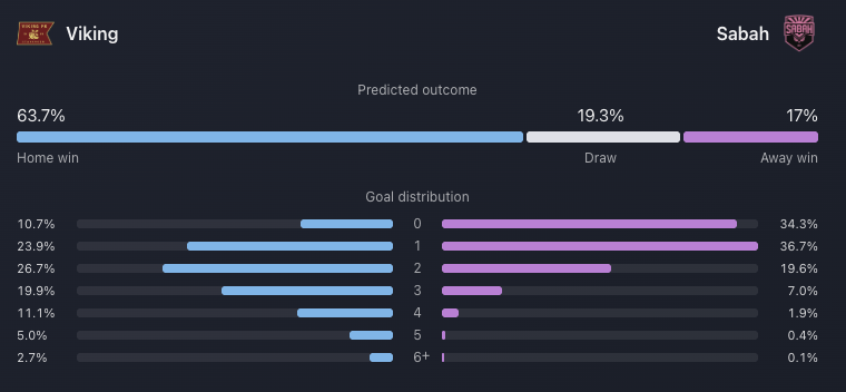
Viking-Sabah projection showing outcome and goal probabilities — Match projection for Viking against Sabah. The top bar shows the probabilities of a home win, draw, and away win. The lower bars show the probability of each side scoring zero to six or more goals.

We began with two domestic records that were difficult to read side by side. The shared scale shows Viking as the stronger club at both ends and clear favourites at home, while Sabah's domestic title gains context from the level of the opposition behind it. The model does not replace scouting or tell us how the match will unfold. It gives match analysis and player evaluation a consistent place to start.

Slik modellerer vi styrken til et fotballag